4.2. RTL Preprocessing
In our design methodology, RTL design is modeled by Finite State Machine with Data (FSMD) which finite state machine model with assignment statements added to each states. The FSMD can completely specify the behavior of an arbitrary RTL design.
In this tutorial, we use an intermediate representation, super finite state machine with data (SFSMD), where each state may take more than one cycle to execute. The SFSMD will be automatically refined into cycle-accurate FSMD after RTL scheduling and binding.
4.2.1. View behavioral input model

Before we show how to generate SFSMD, we take a look at how input model of custom hardware design. Select the behavior "Build_Code" by left clicking on it. We can take a look at the behavioral input model by selecting View->Source from the menu bar.
4.2.1.1. View behavioral input model (cont'd)
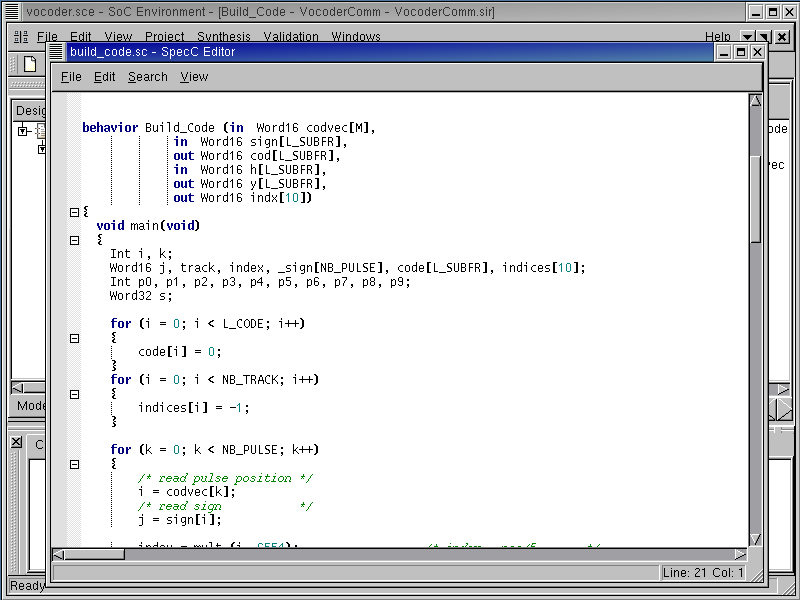
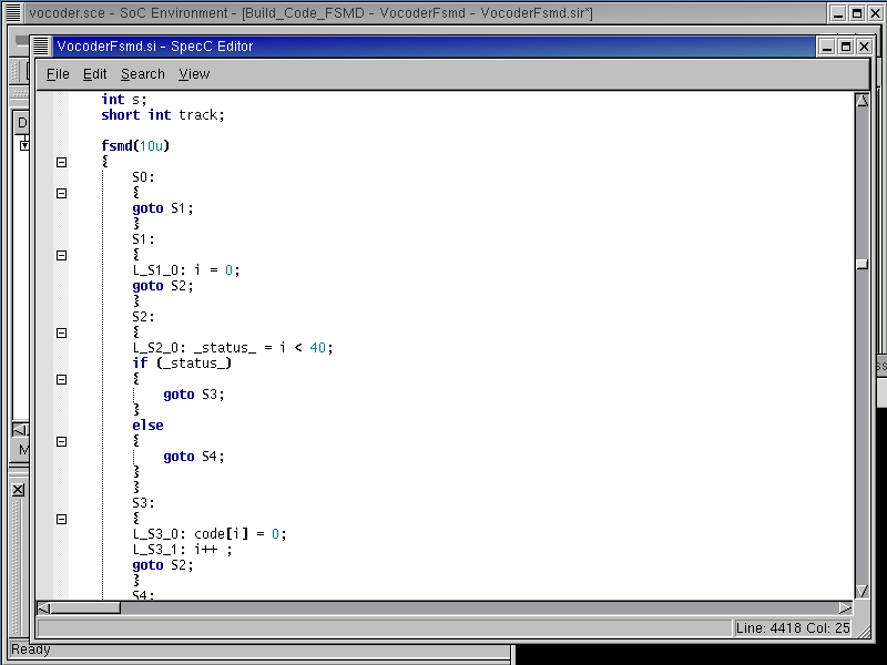
The SpecC Editor window pops up showing the source code for behavior "Build_Code".
4.2.1.2. View behavioral input model (cont'd)

Scrolling down the window, we can see that the behavior code has loops and conditional branch constructs. Therefore, our RTL synthesis tool has to handle these constructs. Close the SpecC Editor window by selecting File->Close from its menu bar.
4.2.2. Generate SFSMD model
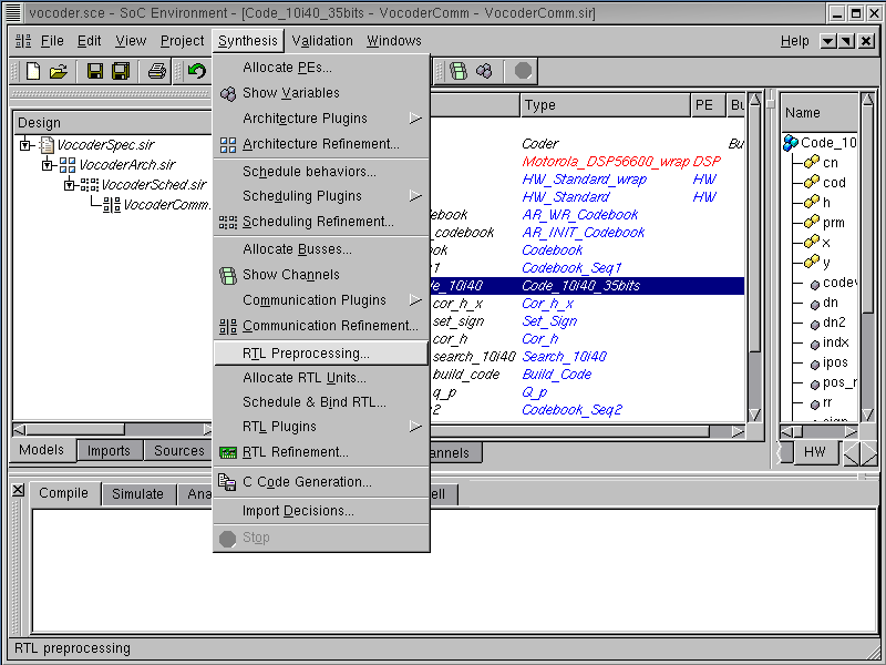
Now, we will show how to generate super finite state machine with data (SFSMD). To demonstrate the features of the our custom hardware synthesis tool, we will use a particular behavior called "Code_10i40_35bits". Browse the hierarchy in the design hierarchy window and select behavior "Code_10i40_35bits". We will be demonstrating RTL design exploration with this behavior in the rest of the chapter.
In the SCE, the step of generating the SFSMD from the behavioral input model is called RTL preprocessing, which is necessary for RTL synthesis. RTL preprocessing can be invoked by selecting Synthesis->RTL Preprocessing from the menu bar.
4.2.2.1. Generate SFSMD model (cont'd)

An RTL Preprocessing dialog box pops up for selecting the behavior and its clock period. Select "Code_10i40_35bits" as the behavior to be preprocessed and leave the default clock period of the behavior as 10 ns. Note that the clock period here is used only for generating a simulatable FSMD construct in SpecC. It does not mean that each state in the SFSMD model will eventually take 10 ns to execute.
In the dialog box, the option Keep original behavior means that the original behavior definitions for "Code_10i40_35bits" and its sub-behaviors will be preserved in the model. Their instances, however, will be replaced by the generated SFSMD behavior instances in the hierarchy.
Now click Start to begin preprocessing.
4.2.2.2. Generate SFSMD model (cont'd)

Note that RTL preprocessing step generates new SFSMDs for 6 sub-behaviors in the behavior "Code_10i40_35bits", as seen on the logging window. Also note that a new model "VocoderComm.fsmd.sir" is added in the project manager window. This new model contains SFSMD behaviors mapped to HW component, which can be seen in the design hierarchy tree.
Again, we must give our new model a suitable name. We can do this by right clicking on "VocoderComm.fsmd.sir" and selecting Rename from the pop up menu. Rename the model to "VocoderFsmd.sir".
4.2.3. Browse SFSMD model
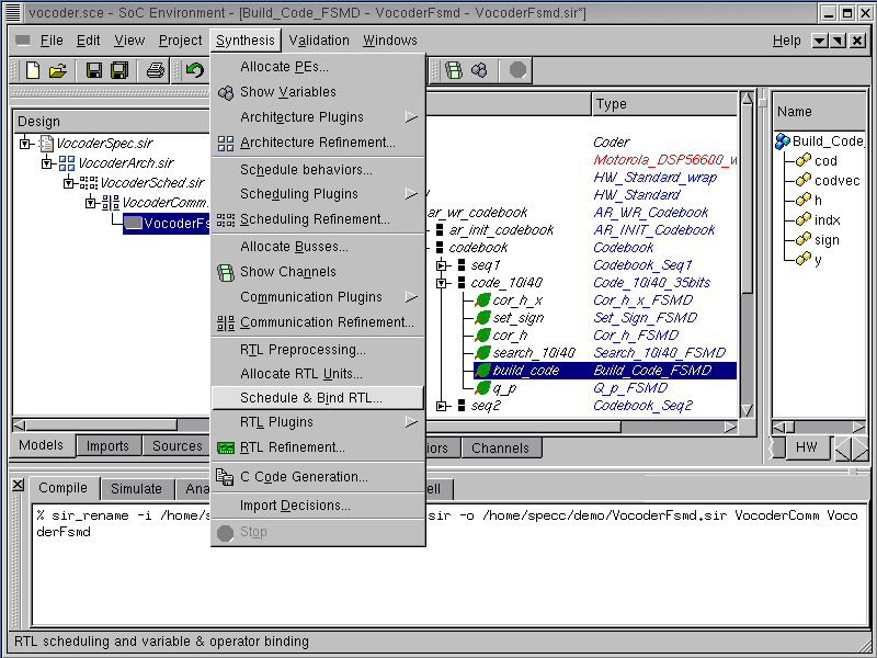
Select the behavior "Build_Code_FSMD" from the hierarchy by left clicking on it. The generated SFSMD leaf behaviors may be viewed by selecting Synthesis->Schedule & Bind RTL from the menu bar.
4.2.3.1. Browse SFSMD model (cont'd)

The RTL Scheduling & Binding window pops up showing all the states in the behavior "Build_Code_FSMD". It also shows all statements for the selected state in the right-most column. We can go inside each state by clicking on the corresponding circle in the left-most column. In this screen shot, state S9 is selected. We can see all assignments with operations and state transitions derived from "if" statements.
Left click on Cancel to close RTL Scheduling & Binding window.
4.2.4. View SFSMD model (optional)
We browsed through the newly created model in the RTL Scheduling & Binding window. In addition, we can also view the source code of the model. Note that if reader is not interested, she or he can skip this section to go directly Section 4.2.5.
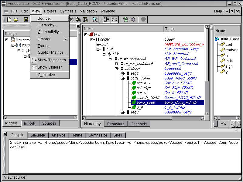
Select behavior "Build_Code_FSMD" by left clicking on it. We now take a look at the source code to see if the RTL preprocessing tool has correctly generated the SFSMD model. Do this by selecting View->Source from the menu bar.
4.2.4.1. View SFSMD model (optional) (cont'd)

The SpecC Editor window pops up showing the source code for behavior "Build_Code_FSMD".
4.2.4.2. View SFSMD model (optional) (cont'd)
The behavioral input model is changed to the SFSMD model with clock period 10 ns. Scroll down the window to find loops and conditional branch constructs in the behavioral input model are changed to state transitions. Still, each state has a lot of assignments and operations, which have to be scheduled and bound.
Close the SpecC Editor window by selecting File->Close from the menu bar.
4.2.5. Simulate SFSMD model (optional)
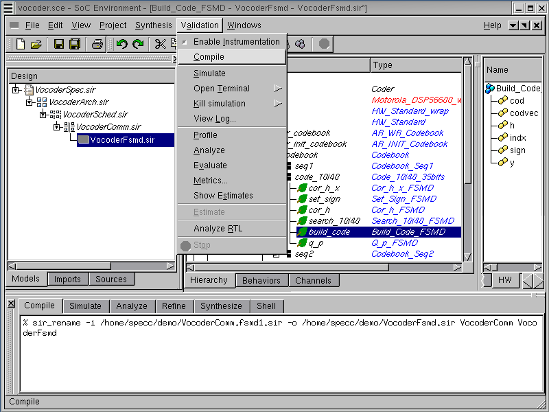
For demo purposes, we will skip the SFSMD generation of those other behaviors assigned to HW component. Even this partially refined model is actually simulatable. To show this, first compile the model by selecting Validation->Compile from the menu bar.
If reader is not interested, she or he can skip this section to go directly Section 4.2.6.
4.2.5.1. Simulate SFSMD model (optional) (cont'd)
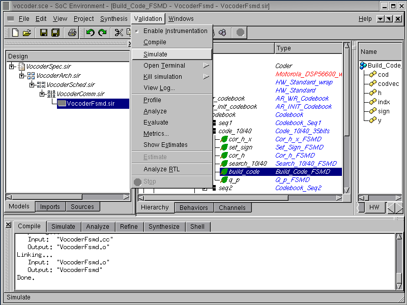
Note that the SFSMD model compiles correctly into executable "VocoderFSMD" as seen in the logging window. We now proceed to simulate the model by selecting Validation->Simulate from the menu bar.
4.2.5.2. Simulate SFSMD model (optional) (cont'd)
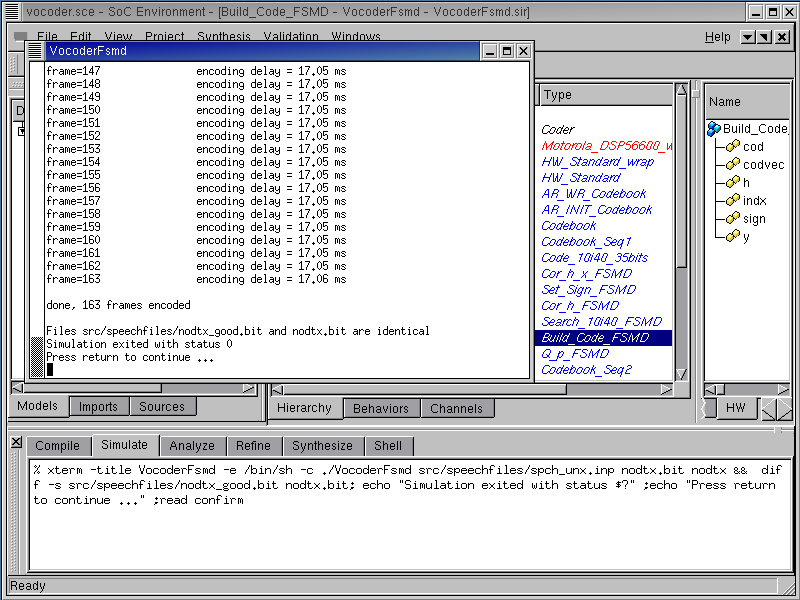
The simulation window pops up showing the progress and successful completion of simulation. We are thus ensured that the SFSMD generation step has taken place correctly. Also note that we can perform the SFSMD generation on any behavior of our choice. This indicates that the user has complete freedom of delving into one behavior at a time and testing it thoroughly. Since the other behaviors are at higher level of abstraction, the simulation speed is much faster than the situation when the entire model is synthesized. This is a big advantage with our methodology and it enables partial simulation of the design. The designer does not have to refine the entire design to simulate just one behavior in RTL.
In this simulation, we see the delay per frame in the SFSMD model decreases to 17.05 ns from 19.89 ns compared to the communication model. Because each state in the SFSMD model is artificially assigned a 10 ns clock period even though it has a lot of assignments and operations to be split into multiple states by scheduling and binding.
4.2.6. Analyze SFSMD model
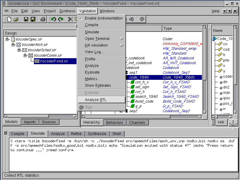
Once the SFSMD model is generated, we need to allocate RTL components. For allocation, we need to get some statistical information on design. The statistical information contains the number of operations for functional unit allocation, the number of live variables for storage unit allocation and the number of data transfers for bus allocation and the number of operations in critical path in each state. These kind of useful information can be obtained by performing RTL analysis. First we select the behavior "Code_10i40_35bits", of which we want to get the statistical information. The RTL analysis is performed by selecting Validation->Analyze RTL from the menu bar.
4.2.6.1. Analyze SFSMD model (cont'd)

RTL analysis tool goes over all sub-behaviors in the behavior "Code_10i40_35bits", and generates their statistical information for the allocation.
4.2.6.2. Analyze SFSMD model (cont'd)
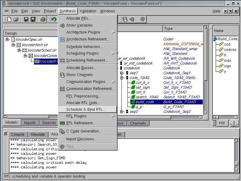
In order to look at RTL analysis result for the behavior "Build_Code_FSMD", select Synthesis->Schedule & Bind RTL from the menu bar.
4.2.6.3. Analyze SFSMD model (cont'd)
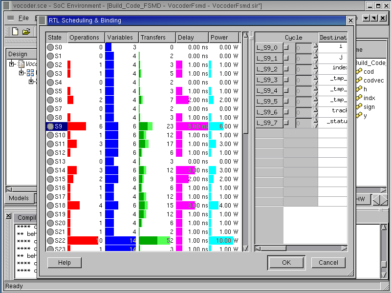
The RTL Scheduling & Binding window pops up showing the statistical information for the selected behavior. From left to right in the left panel of the RTL Scheduling & Binding window, it shows number of operations (Operations column) in each state, number of variables (Variables), number of data transfers (Transfers), number of operations in critical path (Delay), and power dissipation (Power).
4.2.6.4. Analyze SFSMD model (cont'd)
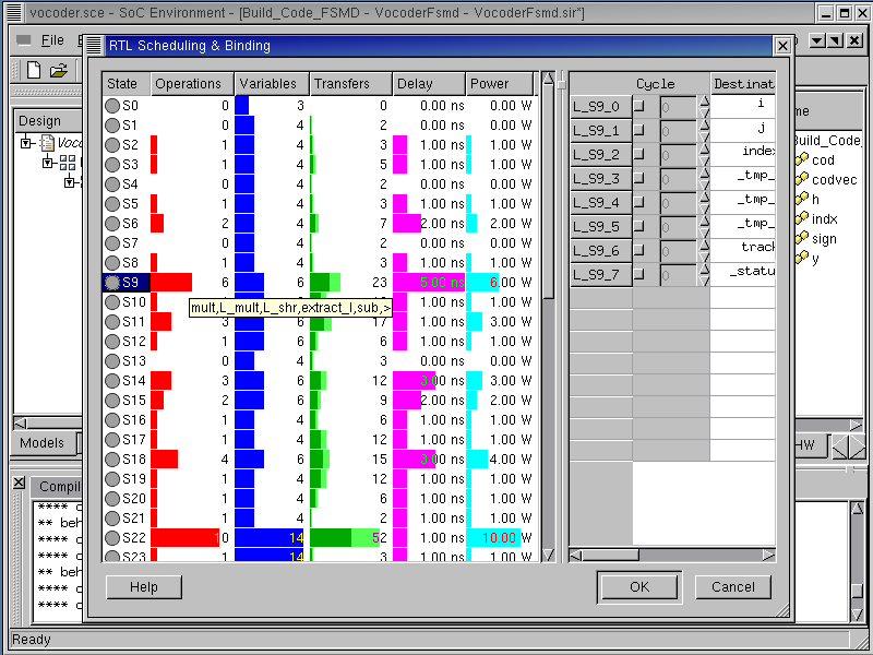
Moving the mouse over the bars in the graph gives us detailed information on each category. For instance, if we put the mouse over the Operations column in each state, the operations which are executed in the state will be shown like mult, L_mult, L_shr, extract_l, sub and > in state S9.
4.2.6.5. Analyze SFSMD model (cont'd)

If we move the mouse over the Variables column in each state, the variables which are live at the end of the state will be shown like code, i, index, indices, k, and track in state S9.
4.2.6.6. Analyze SFSMD model (cont'd)

If we move the mouse over the Transfers column in each state, the data transfers happens at the state will be shown. In state S9, the number of read transfers is 15 and the number of write transfers, 8.
Left click on Cancel to close the RTL Scheduling & Binding.