3.3. Software Scheduling and RTOS Model Insertion
The next step in the system level design process is the serialization of behavior execution on the processing elements. Processing elements (PEs) have a single thread of control only. Therefore, behaviors mapped to the same PE can only execute sequentially and have to be scheduled. Software scheduling and RTOS model insertion is the design step to schedule the behaviors inside each PE.
Depending on the nature of the PE and the data inter-dependencies, behaviors are scheduled statically or dynamically. In a static scheduling approach, behaviors are executed in a fixed and predetermined order, possibly flattening parts of the behavioral hierarchy. In a dynamic scheduling approach on the other hand, the order of execution is determined dynamically during runtime. Behaviors are arranged into potentially concurrent tasks. Inside each task, behaviors are executed sequentially. A RTOS model is inserted into the design. The RTOS model maintains a pool of task behaviors and dynamically selects a task to execute according to its scheduling algorithm. In this chapter we see how we make scheduling decisions using SCE.
3.3.1. Serialize behaviors
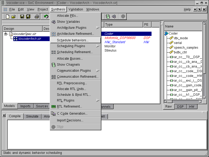
To start behavior scheduling, select Synthesis->Schedule behaviors from the menu bar.
3.3.1.1. Schedule software
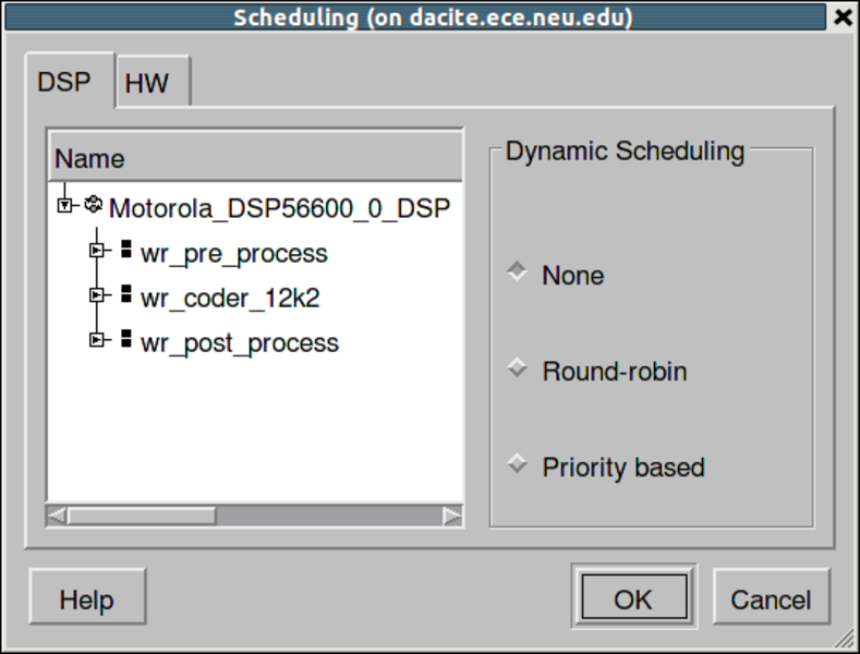
A Scheduling window will pop up. This window includes scheduling options for two PEs (DSP and HW). We begin by selecting the scheduling algorithm for the software. We can do either static scheduling or dynamic scheduling for the software. In case of dynamic scheduling, a RTOS model corresponding to the selected scheduling strategy is imported from the library and instantiated in the PE. The RTOS model provides an abstraction of the key features that define a dynamic scheduling behavior independent of any specific RTOS implementation. SCE provides two RTOS models with different dynamic scheduling algorithms: round-robin and priority based.
3.3.1.2. Schedule software (cont'd)
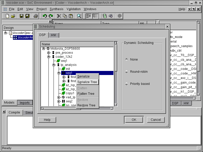
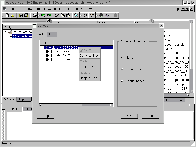
Behavior scheduling is done by converting all concurrent SpecC "par" or "pipe" statements into sequential statements. This conversion is achieved by performing the "serialize" operations on the intended behaviors. For example, assume that behavior "A" is a "par" composition of behavior "B" and "C". With a "serialize" operation, behavior "A" will be changed to a sequential execution of "B" and "C" by default. Another kind of operations, "flatten" are often performed during behavior scheduling to change the behavior hierarchy. Continuing with our example, if behavior "B" itself is composed of "D" and "E" in parallel, a "flatten" operation on "B" removes "B" from "A" while promoting its sub-behaviors, "D" and "E" one level up. As the result, behavior "A" becomes a "par" composition of "D", "E" and "C". Note that the hierarchy relation among behaviors is most conveniently represented as a tree, operations "serialize tree" and "flatten tree" are also provided by SCE to serialize or flatten behaviors of a subtree recursively.
In our design, for example, to serialize the sub-behaviors of behavior "seq1", in the design hierarchy tree, select behavior "seq1". Right click to bring up a menu window and select Serialize Tree from the menu.
3.3.1.3. Schedule software (cont'd)
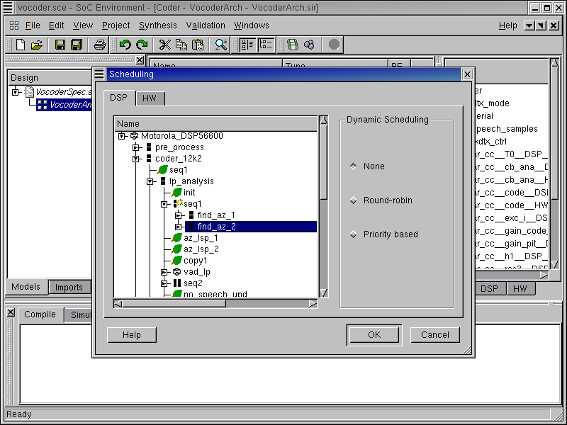
Now that the two parallel child behaviors of behavior "seq1": behavior "find_az_1" and behavior "find_az_2" are converted into two sequential behaviors. We can see that behavior "find_az_1" is executed before behavior "find_az_2". This execution order is created by the tool. The designer can modify the execution order.
3.3.1.4. Schedule software (cont'd)
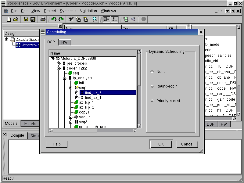
Select behavior "find_az_2". Left click and move behavior "find_az_2" before behavior "find_az_1". Now behavior "find_az_2" is executed before "find_az_1". In general, the designer can specify any "par" or "pipe" statements to be scheduled and manually specify the execution order of any parallel behaviors in the same level. The remaining parallel behaviors can either be dynamically scheduled by the RTOS model or statically serialized by the tool.
Since we want the tool to schedule all the behaviors automatically, we restore the execution order created by the tool. Select behavior "find_az_1". Left click and move behavior "find_az_1" before behavior "find_az_2".
3.3.1.5. Schedule software (cont'd)
For our example, since there are not many parallel behaviors in DSP, we statically schedule the behaviors in DSP. In the dynamic scheduling box, click and select None.
Also, we will leave the decision of behavior execution order to be made automatically by the tool. In the design hierarchy tree, select behavior "Motorola_DSP56600". Right click and select Serialize Tree.
3.3.1.6. Schedule software (cont'd)
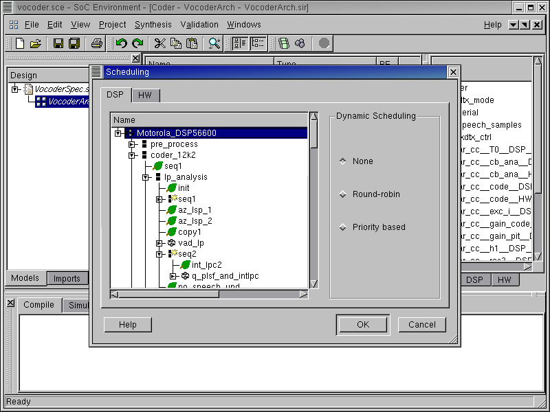
As shown in the figure, all the child behaviors of behavior "Motorola_DSP56600" are serialized. Behaviors that are modified as a result of serialization are marked with a "*" symbol next to them.
3.3.1.7. Serialize behaviors in HW
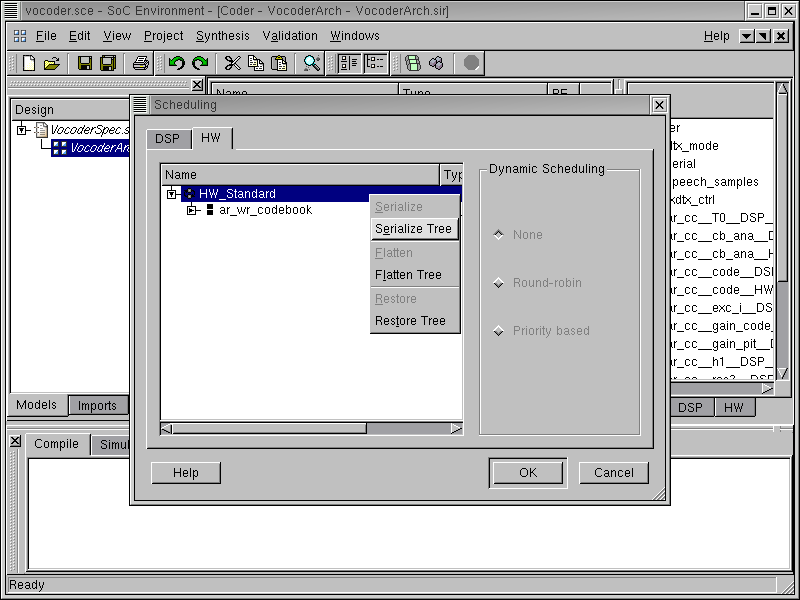
The next step is to serialize behaviors in HW. Since custom hardware can only be statically scheduled, the dynamic scheduling box is disabled for HW. Click and select HW in the Scheduling window. In the design hierarchy tree, select behavior "HW_Standard". Right click and select Serialize Tree.
3.3.1.8. Serialize behaviors in HW (cont'd)
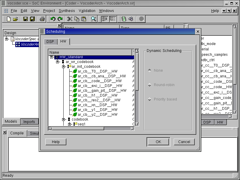
As shown in the figure, all the child behaviors of behavior "HW_Standard" are serialized. Click OK button to confirm the scheduling decision.
3.3.2. Generate serialized model

Once the scheduling decisions have been made, we can refine the architecture model to reflect the changes. A software scheduling and RTOS model insertion tool is integrated in SCE. The tool will generate the model to reflect the scheduling algorithm we selected. In case of dynamic scheduling, a RTOS model is inserted into the design and behaviors are converted into tasks with assigned priorities. To invoke the tool, go to Synthesis menu and select Scheduling Refinement.
3.3.2.1. Refine after serialization
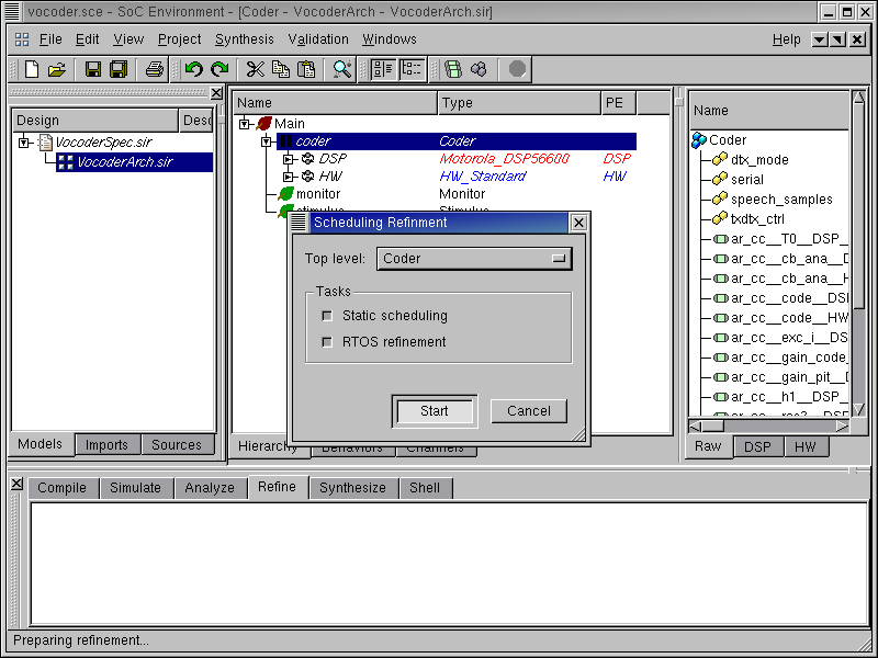
A dialog box pops up for selecting specific refinement tasks. By default, all tasks will be performed in one go. Press the Start button to start the refinement.
It must be noted that the user has an option to do the refinement tasks one step at a time. For instance, a designer may select only static scheduling if he or she is not concerned about observing the dynamic scheduling behavior on the component.
3.3.2.2. Refine after serialization (cont'd)

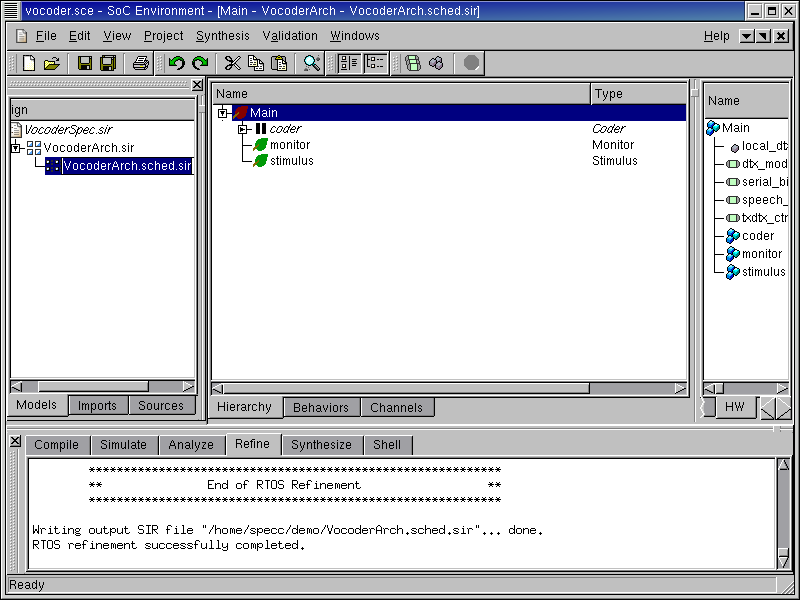
The logging window shows the refinement process. After the refinement, the newly generated serialized model "VocoderArch.sched.sir" is displayed to the design window. It is also added to the current project window, under the architecture model "VocoderArch.sir" to indicate that it was derived from "VocoderArch.sir".
3.3.2.3. Refine after serialization (cont'd)
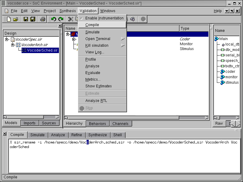
As we did for previous models, we change the name of the serialized architecture model to "VocoderSched.sir" in the project window.
3.3.3. Simulate serialized model (optional)
This section shows the simulation of the generated model. If the reader is not interested, she or he can skip this section and go directly to Section 3.4.
Serialization refinement is now complete with the generation of a new model. However, we also need to confirm that the model has not lost any of its functionality in the refinement process. In other words the new model must be functionally equivalent to the architecture model.
We will validate the serialized architecture model through simulation. But first we need to compile the model into an executable. To compile the serialized architecture model to executable, go to Validation menu and select Compile.
3.3.3.1. Simulate serialized model (optional) (cont'd)
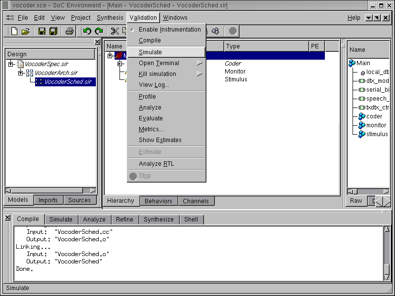
The messages in the logging window shows that the refined model is compiled successfully without any errors. Now in order to verify that it is functionally equivalent to the architecture model, we will simulate the compiled model on the same set of speech data used in the specification validation. Go to Validation menu and select Simulate.
3.3.3.2. Simulate serialized model (optional) (cont'd)
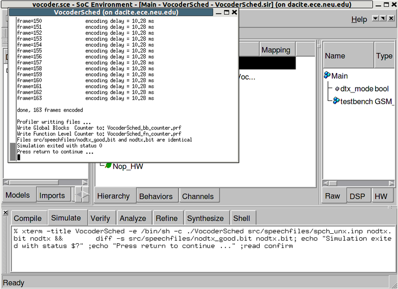
The simulation run is displayed in a new terminal window. As we can see, the serialized architecture model was simulated successfully for all 163 frames of speech data. The result bit file is also compared with the expected golden output given with the Vocoder standard. We have thus verified that the generated refined model is functionally correct. Note that the execution time for each frame now becomes 10.28 ms. Recall that the execution time was 8.81 ms for each frame before the software scheduling is performed. The increase of execution time is reasonable since the concurrency in the previous model is removed by the software scheduling.