3.2. Architecture Exploration
Architecture exploration is the design step to find the system level architecture and map different parts of the specification to the allocated system components under design constraints. It consists of the tasks of selecting the target set of components, mapping behaviors to the selected components and implementing correct synchronization between the components. Note that the components themselves are independent entities that execute in a parallel composition. In order to maintain the original semantics of the specification, the components need to be synchronized as necessary. Architecture exploration is usually an iterative process, where different candidate architectures and mappings are experimented to search for a satisfactory solution.
As indicated earlier, the timing constraint for the Vocoder design is the real time response requirement, i.e., the time to encode and decode the speech should be less than the speech time. The test speech has a 3.26 seconds duration. Therefore, the final implementation must meet this time constraint. In this chapter we see how we arrive at a suitable architecture with keeping this requirement in mind and using the refinement tool.
3.2.1. Try pure software implementation
The goal of our exploration process is to implement the given functionality on a minimal cost architecture and still meet the timing constraint. The first approach is to implement everything in software so that we do not have the overhead of adding extra hardware and associated interfaces. To accomplish this, we first select a processor out of our component database. Thereafter, we map the entire specification on to this processor. Once the mapping is done, we invoke the analysis tool to see if the processor alone is sufficient to implement the system.
3.2.1.1. Try pure software implementation (cont'd)
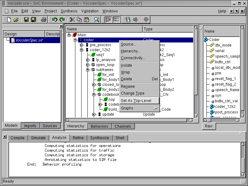
Before we move on, the top level behavior of the design needs to be specified. This is necessary because the specification model may have some test bench behaviors, which are not going to be included in the final design. It may be recalled that the project we are working with involves not only the design-under-test (DUT) but also the behaviors that drive it. For example, the behaviors "Monitor" and "Stimilus" are just testbench behaviors while the behavior "Coder" represents the real design. To specify "Coder" as the top level behavior, right click on "Coder" to bring up a drop box menu then left click on Set As Top-Level.
3.2.1.2. Try pure software implementation (cont'd)
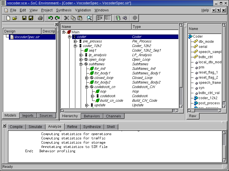
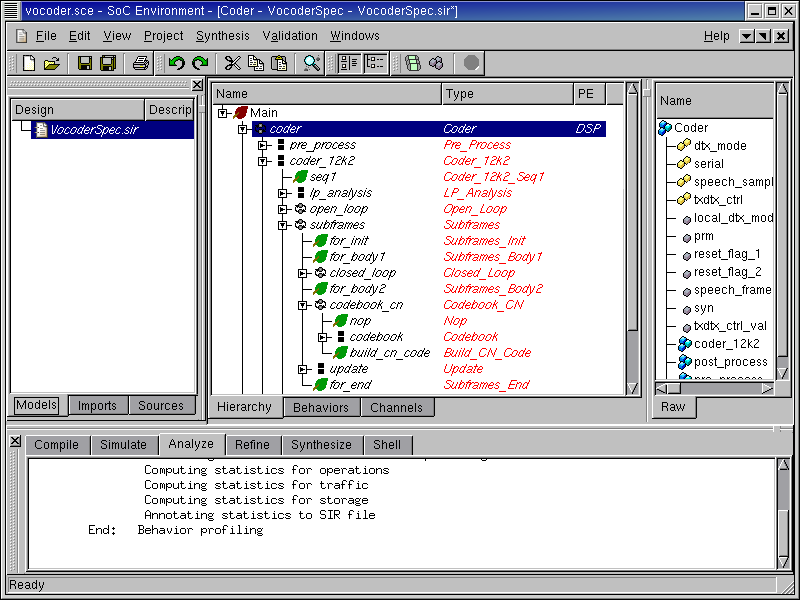
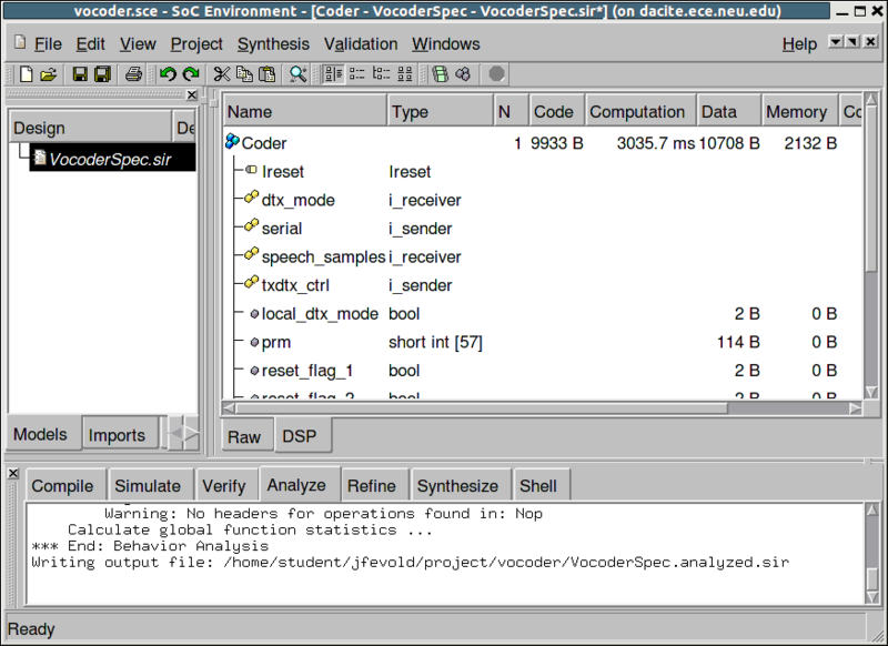
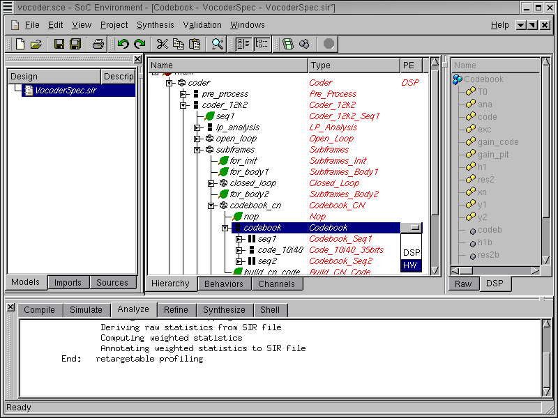
As shown in the figure, when the top level behavior "Coder" is specified, the names of all its child behaviors are italicized to distinguish them from the test bench behaviors. In general, any behavior which needs to be tested can be set as top level. So, in a generic sense, the design under test can be identified by the italicized font.
3.2.1.3. Try pure software implementation (cont'd)
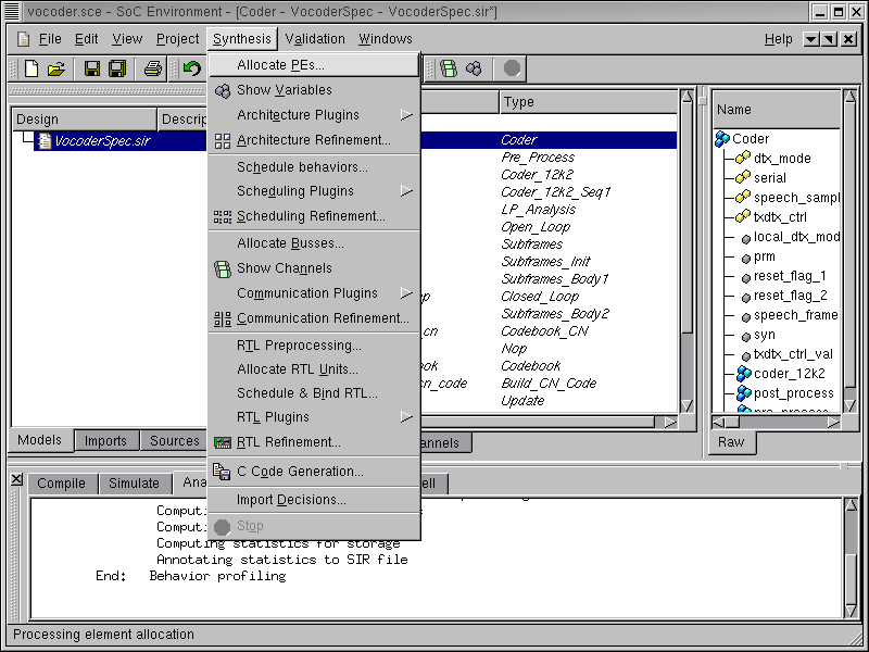
We begin by exploring the available set of components in the database. This is required to select a suitable processor. To view all available components and select the desired processor, select Synthesis->Allocate PEs... from the menu bar.
3.2.1.4. Try pure software implementation (cont'd)
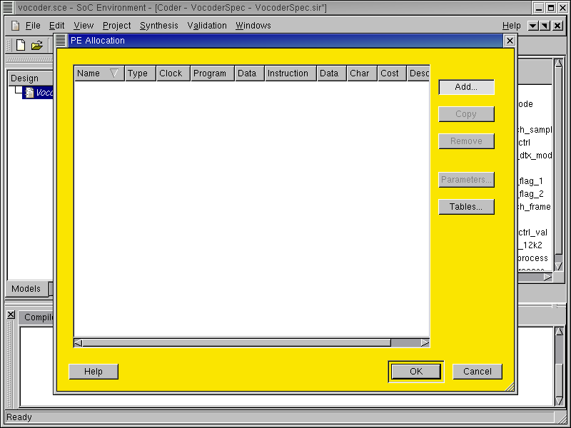
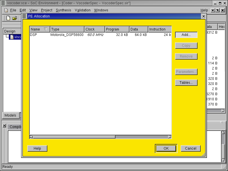
Now a PE Allocation window pops up. This window includes a table to display important characteristics of components selected for the design. In addition, it also provides a number of buttons (on the right side) for user actions, such as adding a component, removing a component, and so on. Since we have not allocated any component at this point, the table has no entry.
To view the component database and select the desired component, press the Add... button.
3.2.1.5. Try pure software implementation (cont'd)
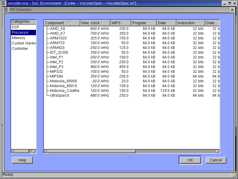
Now a PE Selection window is brought up. The left side of the window (Categories) lists five categories of components stored in the database. The right side of the window displays all components within a specific category along with their characteristics. As shown in the above figure, since the Processor category is selected on the left side, 15 commonly used processor components are displayed in detail on the right side.
The Component description includes features like maximum clock speed, measure of the number of instructions per second, a cost metric, cache sizes, instruction and data widths and so on. These metrics are used for selecting the right component. Remember that the profiling data has given us an idea of what kind of component would be suitable for the application at hand.
3.2.1.6. Try pure software implementation (cont'd)
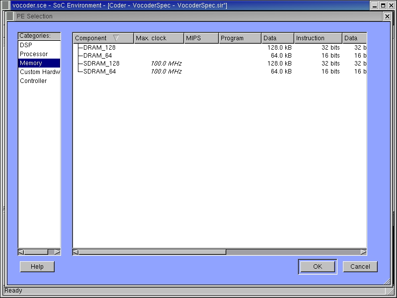
Now if we go to the Mem category, a number of memory components will be displayed in detail on the right side of the window. If the memory in the processor is insufficient for the application, we can add external memory components from this table.
3.2.1.7. Try pure software implementation (cont'd)
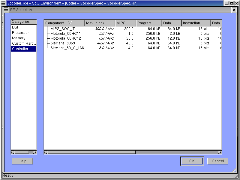
Now if we go to the Controller category, a number of widely used micro-controller components will be displayed in detail on the right side of the window.
3.2.1.8. Try pure software implementation (cont'd)
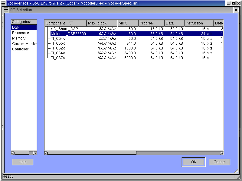
Through earlier profiling and analyzing, we found out that integer multiplication is the most significant operations in the original specification. Therefore, a fixed-point DSP would be desirable for this design.
Under the DSP category, a number of commercially available DSPs are displayed. These DSP components are maintained as part of the component library and may be imported into the design upon requirement. Since the Vocoder design project was supported by Motorola, our first choice is DSP56600 from Motorola.
Left click the "Motorola_DSP56600" row to select it. Then click OK button to confirm the selection.
3.2.1.9. Try pure software implementation (cont'd)
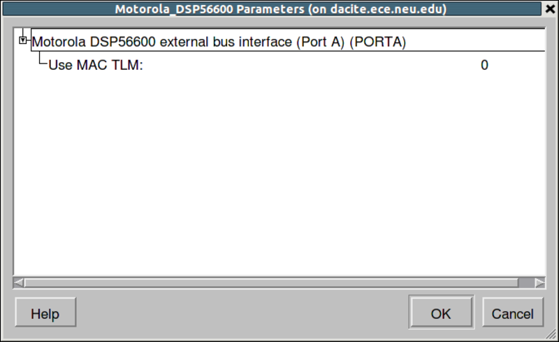
After clicking OK to confirm the selection in the PE Selection dialog, a new dialog will pop up to allow entering parameters of the allocated Motorola DSP. Use the default parameters, i.e., accept the dialog by clicking OK.
3.2.1.10. Try pure software implementation (cont'd)
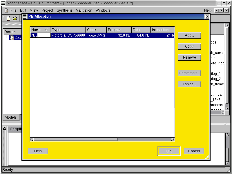
Now the PE Selection window goes away and the PE Allocation table has one row that corresponds to our selected component, which has a type of "Motorola_DSP56600". This new component was named as "PE0" by default. To make it more descriptive for later reference, it is desirable to rename it.
To rename it, just left click in the Name column of the row. The cursor will be blinking to indicated that the text field is ready for editing.
3.2.1.11. Try pure software implementation (cont'd)
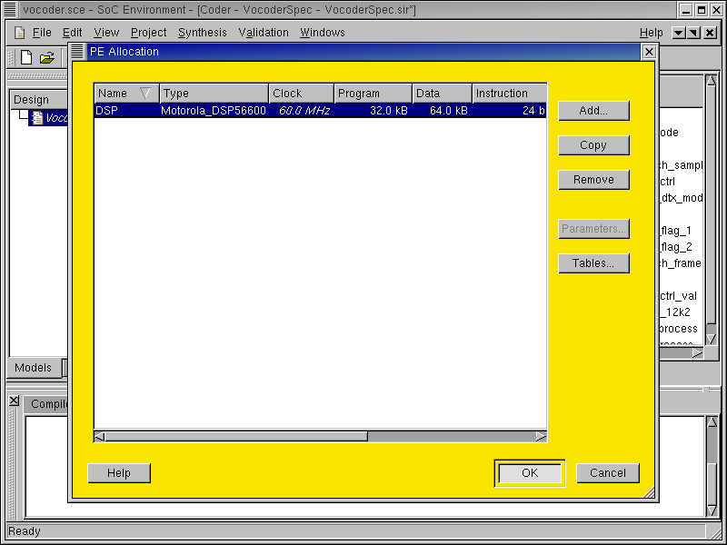
We will simply name the component as "DSP" since it is the only component used in the design at this instance. Proceed by typing "DSP" in the text field and press return to complete the editing. Then press the OK to finish component allocation.
3.2.1.12. Try pure software implementation (cont'd)
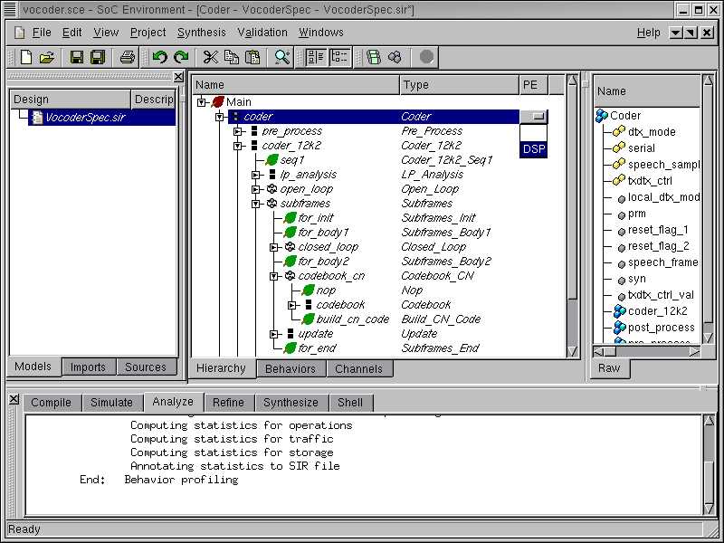
As mentioned earlier, we will map the whole design to the selected processor. This is done by assign the top level behavior "Coder" to "DSP". Left click in the PE column in the row for the "Coder" behavior. A drop box containing allocated components comes up. Left click on "DSP" to map behavior "Coder" to "DSP".
It should be noted that any kind of mapping is allowed. However, since we are investigating a purely software implementation, everything in the design gets mapped to the "DSP".
3.2.1.13. Try pure software implementation (cont'd)
As we can see now, the descendant behaviors are all highlighted in red to indicated that they are mapped to the "DSP" component.
3.2.2. Estimate performance
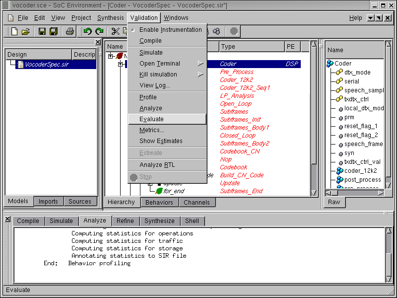
The next step is to analyze the performance of this architecture. Recall that we have a timing constraint to meet. We must therefore check if a purely software implementation would still suffice. If not, we will try some other architecture. Now we can estimate the performance of this pure software mapping by selecting Validation->Evaluate from the menu bar.
3.2.2.1. Estimate performance (cont'd)
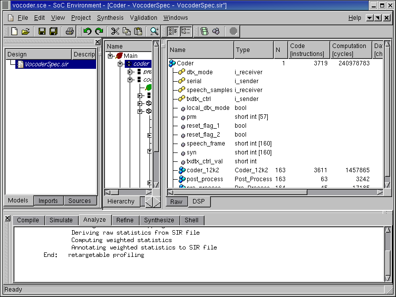
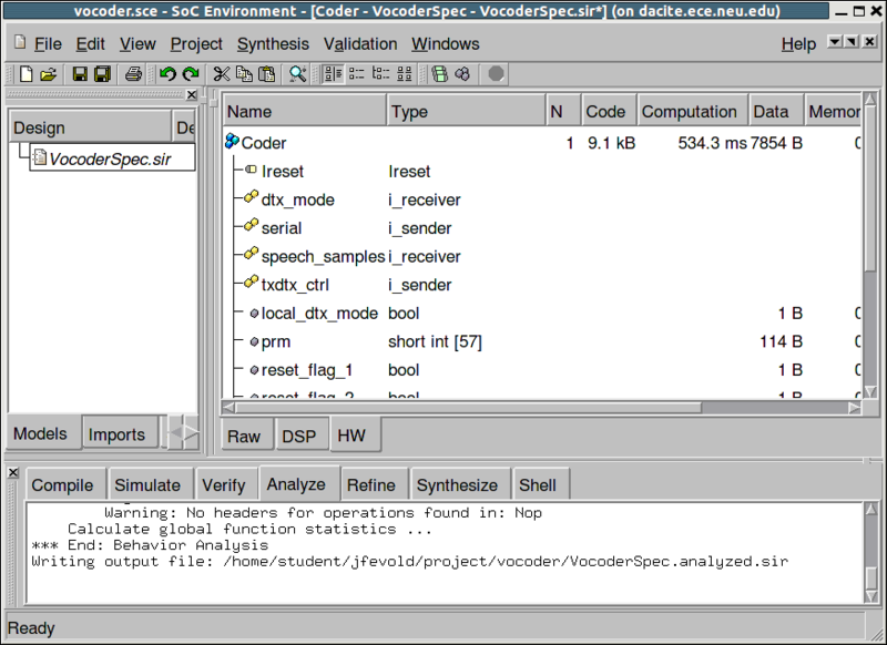
As we can see in the logging window, a re-targeted profiling is being performed. Notice in the log information that raw statistic generated during profiling are used here. The raw statistics are take as an input to the analysis tool that generates statistics for the current architecture. Since, we know the parameters of the DSP, the analysis tool can provide a more accurate measure of actual timing. When that is done, the profiled data is displayed in the design window with the "DSP" tab. Notice that this tab has appeared at the bottom of the design data. The total computation time is shown in terms of number of DSP clock cycles.
3.2.2.2. Estimate performance (cont'd)
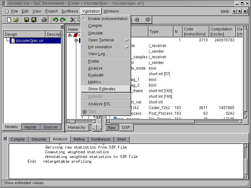
The number of computation cycles is a relevant metric for observation. However, it must be converted to an absolute measure of time so that we may directly verify if this architecture meets the demands. To find out the real execution time in terms of seconds, we turn on the option for estimation by selecting Validation->Show Estimates from the menu bar.
3.2.2.3. Estimate performance (cont'd)
As seen in the design window, the computation time is in unit of "us". As we can see in the row of behavior "Coder", the estimated execution time (~ 4.00 seconds) exceeds the timing constraint of 3.26 seconds.
3.2.2.4. Estimate performance (cont'd)
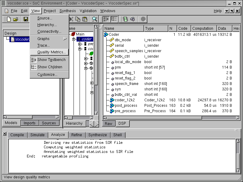
We can also view the design quality metrics such as the execution time by selecting View->Quality Metrics from the menu bar.
3.2.2.5. Estimate performance (cont'd)
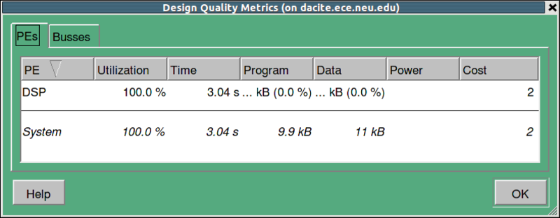
A Design Quality Metrics table pops up, showing that the estimated execution time to be 4.02 seconds, which exceeds the timing constraint of 3.26 seconds. Therefore, the pure software solution with a single "Motorola_DSP56600" does not work. We, therefore, need to experiment with other architectures. To proceed, click OK to close the Design Quality Metrics table.
3.2.3. Try software/hardware implementation
From what we observed while studying the vocoder specification, the design is mostly sequential. There is not much parallelism to exploit. What we need to reduce the execution time is a much faster component than the DSP we used. Some of the critical time consuming tasks may be mapped to a fast hardware. In this iteration, we will try to add one hardware component along with the DSP to implement the design. As we found out earlier, one of the computationally intensive and critical part in the Vocoder is the Codebook behavior. We hope to speed it up by mapping it to a custom hardware component and execute the remaining behaviors on the DSP.
3.2.3.1. Try software/hardware implementation (cont'd)
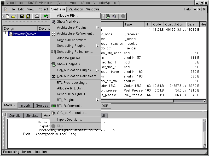
As we did earlier, while selecting the processor, go to Synthesis->Allocate PEs... on the menu bar.
3.2.3.2. Try software/hardware implementation (cont'd)
This time, the PE Allocation table pops up. As we can see, the previously allocated "DSP" component is displayed. To insert the hardware component, press Add... button to go to component database.
3.2.3.3. Try software/hardware implementation (cont'd)
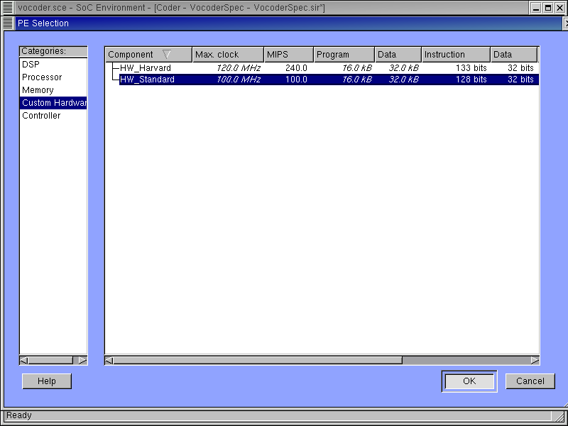
In the Custom Hardware category, two general types of hardware components are displayed. Here we will use the standard hardware design with a datapath and a control unit. Select the "HW_Standard" and press OK to confirm the selection.
3.2.3.4. Try software/hardware implementation (cont'd)
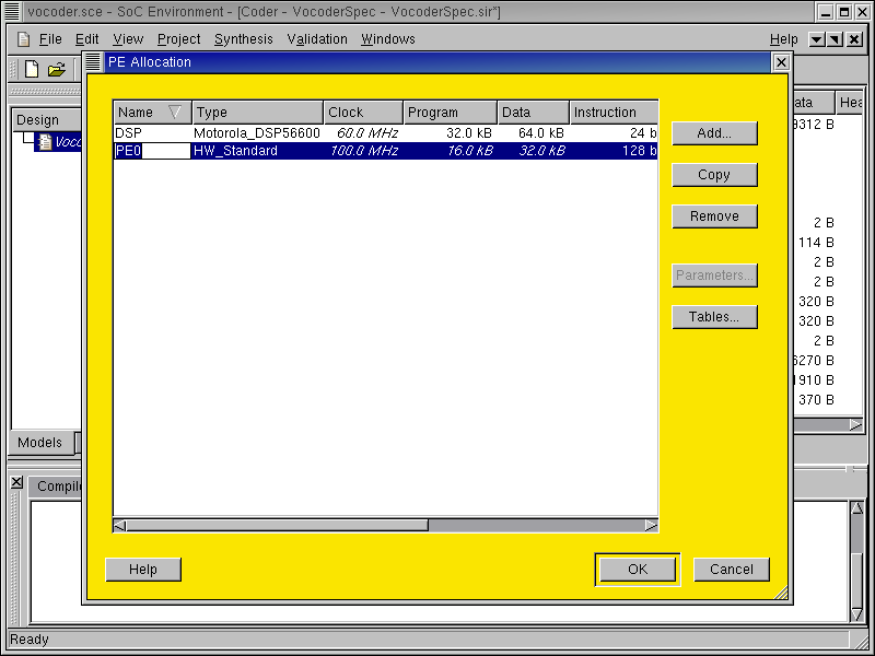
Now the "HW_Standard" component is added to the PE Allocation table. In the same way we did for the "DSP" component, we simply rename it to "HW" to distinguish it. Notice that for the hardware component, some metrics are flexible. For instance, the clock period may be changed. However, we stay with the current speed of 100 Mhz for demo purpose.
3.2.3.5. Try software/hardware implementation (cont'd)
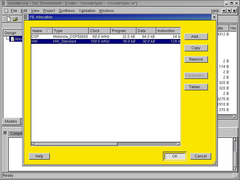
After we renamed it, press OK button to complete component allocation.
3.2.3.6. Try software/hardware implementation (cont'd)
Remember we have already specified the top level behavior and mapped all behaviors to "DSP" in the first iteration. That information is still there and we do not have to specify it again. We only need to map behavior "Codebook" to the "HW" component, as suggested earlier.
Browse the hierarchy tree to locate behavior "Codebook". Click on "Codebook" in the PE column. Click on "HW" in the drop box to map "Codebook" to "HW". This would map the entire subtree of behaviors under "Codebook" to custom hardware.
3.2.3.7. Try software/hardware implementation (cont'd)
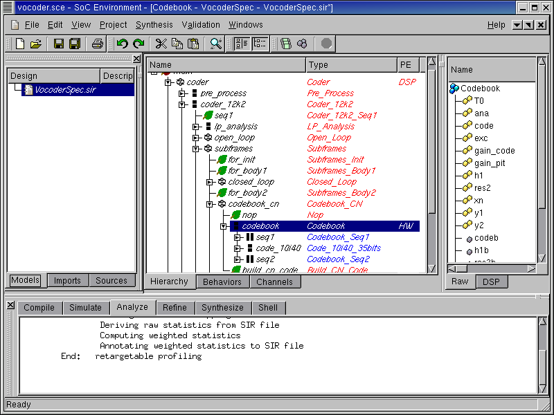
After the mapping, we will see the subtree rooted at "Codebook" is highlighted in blue in contrast to the rest behaviors in red that are mapped to "DSP".
3.2.4. Estimate performance
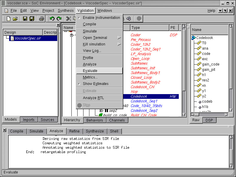
It may be recalled that we abandoned the pure software implementation because it failed on meeting the timing constraint. It is now time for us to verify if the timing is met by using the combined software/hardware design. To evaluate this software and hardware implementation, go to Validation->Evaluate on the menu bar.
3.2.4.1. Estimate performance (cont'd)
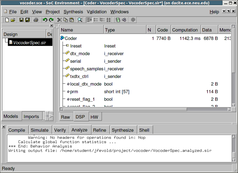
As we can see in the logging window, a profiling re-targeted at the DSP and HW architecture is being performed. When it finishes, the profiled data is presented in the design window. In order to find out the execution time of the Coder, select Coder behavior in the hierarchy tree. By clicking on the DSP tab of the view-pane, information of the DSP part of "Coder" behavior is displayed. For example, the execution time of the software part on DSP is around 1.14 seconds.
3.2.4.2. Estimate performance (cont'd)
To find out the information on hardware side, click the HW tab. The view-pane shows that the execution of hardware part, behavior "Codebook", takes 0.54 seconds. Since "Codebook" was executed in sequential composition with the rest of the design, the latency of the design is the sum of DSP and HW execution time, which is 1.68 (1.14 + 0.54) seconds. Recall that the timing requirement is to be less than 3.26 seconds for the given speech data. Therefore, the current architecture and mapping are acceptable.
3.2.4.3. Estimate performance (cont'd)
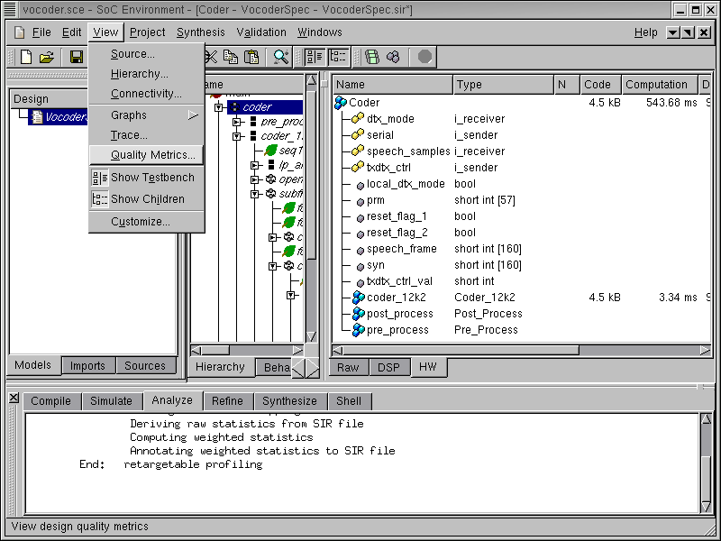
Like we did earlier, we can also view the execution time in the Design Quality Metrics table. To do so, select View->Quality Metrics from the menu bar.
3.2.4.4. Estimate performance (cont'd)
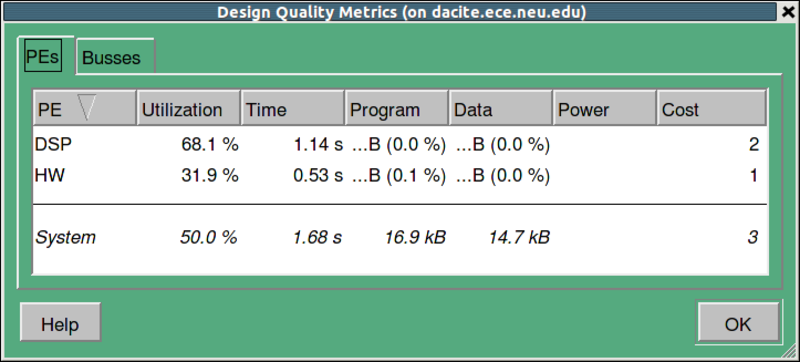
As shown in the figure, the Design Quality Metrics table including a number of design quality metrics is displayed. It confirms that the total execution time is 1.68 seconds, same as what we figured out earlier. After reviewing the quality metrics, click on OK to close the table.
3.2.5. Generate architecture model
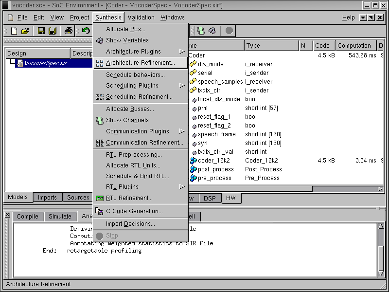
Now we can refine the specification model into an architecture model, which will exactly reflect the this architecture and mapping decisions. This can be done either manually or automatically. As we mentioned earlier, an architecture refinement tool is integrated in SCE. To invoke the tool, go to Synthesis->Architecture Refinement.... The tool changes the model to reflect the partition we created and also introduces synchronization between the parallely executing components. Note that we have not decided to map variables explicitly to components. For demo purposes, we will leave this decision to be made automatically by the refinement tool. However, it needs to be mentioned that the designer may choose to map variables in the design as deemed suitable.
3.2.5.1. Generate architecture model (cont'd)
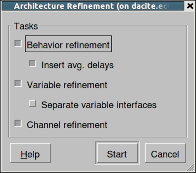
A dialog box pops up for selecting specific refinement tasks of architecture refinement. By default, all tasks will be performed in one go. Now press the Start button to start the refinement. It must be noted that the user has an option to do the architecture refinements one step at a time. For instance, a designer may want to stop at behavior refinement if he is not primarily concerned about observing the memory requirements or the schedule on each component. Nevertheless, in our demo we perform all steps to generate the final architecture model.
3.2.5.2. Generate architecture model (cont'd)
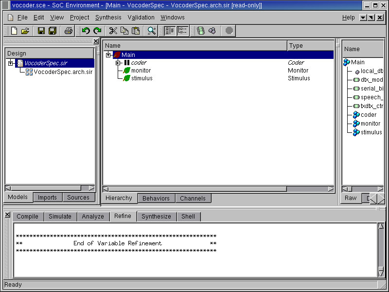
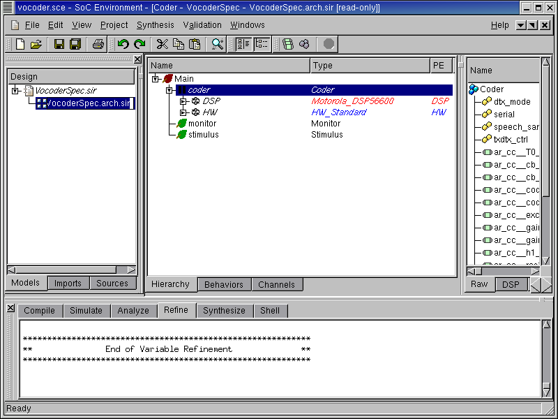
As displayed in the logging window, the architecture refinement is being performed. After the refinement, the newly generated architecture model "VocoderSpec.arch.sir" is displayed to the design window. It is also added to the current project window, under the specification model "VocoderSpec.sir" to indicate that it was derived from "VocoderSpec.sir". Please note that, while the architecture refinement only took a few seconds to generate, a whole new model has been created.
3.2.6. Browse architecture model
In this section we will look at the architecture model to see some of its characteristics.
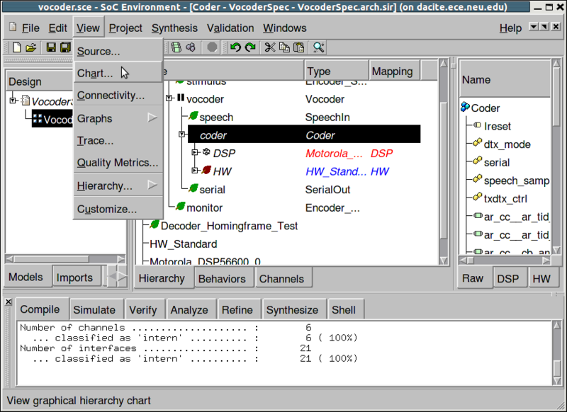
Since the top level behavior is "Coder", the test bench behaviors are not changed during architecture refinement. Therefore let's select "Coder" by clicking in the corresponding row in the design window. We would like to see how the design looks when it is mapped to the selected architecture. To view the hierarchy of the new "Coder" behavior, go to View->Chart.
3.2.6.1. Browse architecture model (cont'd)
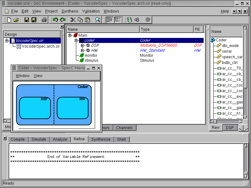
A window pops up, showing all sub-behaviors of the "Coder" behavior. As we can see, this new top level behavior Coder in the architecture model is composed of two new behaviors, "DSP" and "HW", which were constructed and inserted during architecture refinement. These behaviors at the top level indicate the presence of two components selected in the architecture. Note that they are also composed in parallel, which represents the actual semantics of the architecture model.
3.2.6.2. Browse architecture model (cont'd)
We would now like to see how the "DSP" and "HW" behaviors are communicating. This will verify if the refinement process was correctly executed. Go to View->Connectivity to see the connectivity between the "DSP" and the "HW" components.
3.2.6.3. Browse architecture model (cont'd)
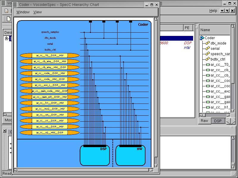
Enlarge the new window and scroll down to view the connectivity of the two components. We can see that "DSP" and "HW" components are connected through global variable channels, which were inserted during the architecture refinement. This is different from the original specification model, where only global variables were used for communication.
After checking the new architecture model, we can close the pop up window and go back to the design window by selecting Window->Close from the menu bar.
3.2.6.4. Rename architecture model
Like what we did for the specification model, we also change the name of the new model to be "VocoderArch.sir" in the project window. The renaming is just for the purpose of maintaining a nomenclature schema and to correctly identify the individual models.
3.2.7. Simulate architecture model (optional)
This section shows the simulation of the generated architecture model. If the reader is not interested, she or he can skip this section and go directly to Section 3.3.
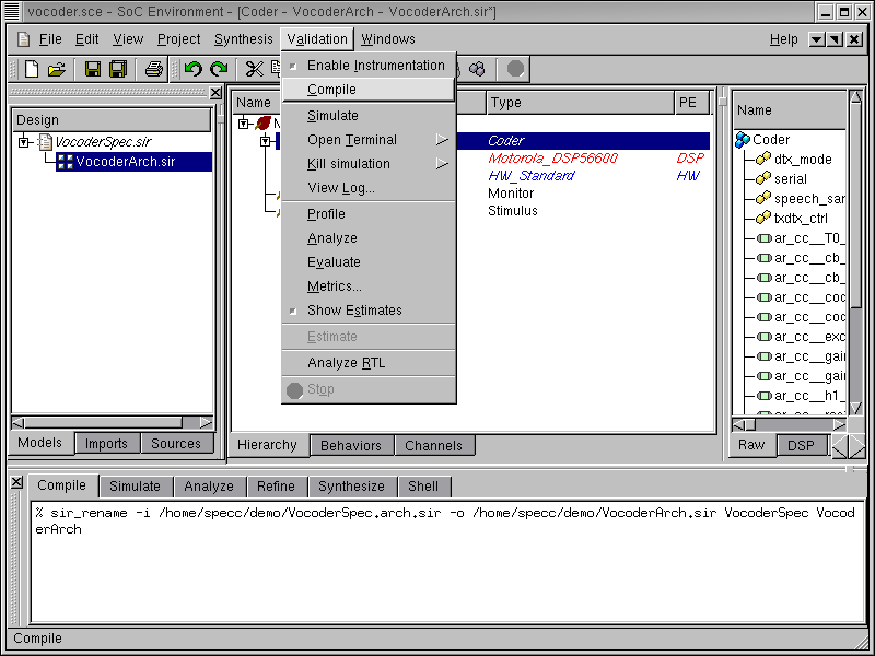
So far we have graphically visualized the automatically generated architecture. We have seen that in terms of its structural composition, the model meets the semantics of an architecture level model in our SoC methodology. However, we also need to confirm that the model has not lost any of its functionality in the refinement process. In other words the new model must be functionally equivalent to the specification. We will validate the architecture model through simulation. But first we need to compile the model into an executable. To compile the architecture model to executable, select Validation->Compile from the menu bar.
3.2.7.1. Simulate architecture model (optional) (cont'd)
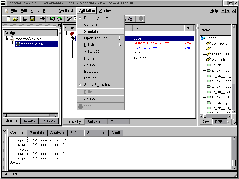
The messages in the logging window show that the architecture model is compiled successfully without any syntax error. Now in order to verify that it is functionally equivalent to the specification model, we will simulate the compiled architecture model on the same set of speech data used in the specification validation by selecting Validation->Simulate from the menu bar.
3.2.7.2. Simulate architecture model (optional) (cont'd)
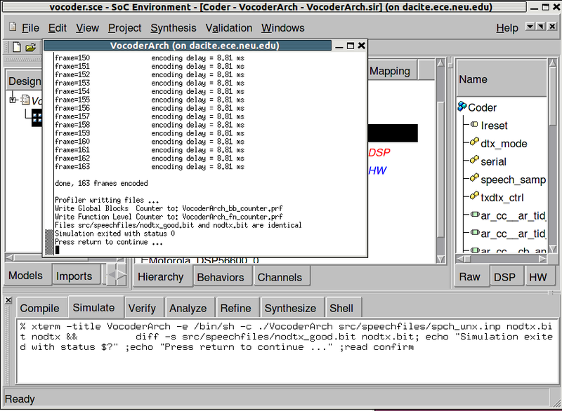
The simulation run is displayed in a new terminal window. As we can see, the architecture model was simulated successfully for all 163 frames speech data. The result bit file is also compared with the expected golden output given with the Vocoder standard. We have thus verified that the generated architecture model is functionally correct. In addition, the simulation of the architecture model shows that the processing time for each frame is 8.81 ms, which was not available when simulating the specification model.
It must be noted as before that the testing process requires fairly intensive execution, but for the demo purposes we will omit multiple simulations and just show the concept. This concludes the step of architecture exploration.