2.3. Simulation and Analysis
Once we have captured the specification as a model and browsed through its behavioral hierarchy and connectivity, we need to ensure that our specification is correct. We also need to analyze our specification model to derive interesting observations about the nature of the computation. The check for correctness is done by simulating the model. Note that the model is purely functional, so the simulation runs very quickly. This is also a good time to debug the model for functional errors that might have crept in while writing it.
After the model is verified to be functionally correct, we proceed to the analysis phase. For this, we need to profile the model using the profiling tool available in SCE. The profile gives us useful information like the about of computation, its distribution over the various behaviors in the model and its nature. This information is need to make crucial architectural choices as we will see as the demo proceeds.
2.3.1. Simulate specification model
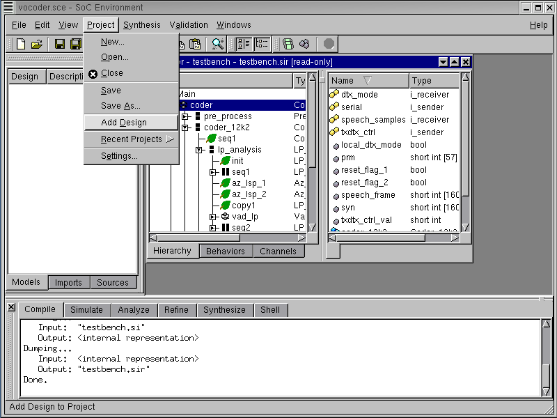
We must now proceed to validate the specification model. Remember that we have a "golden" output for encoding of the 163 frames of speech. The specification model would meet its requirements if we can simulate it to produce an exact match with the golden output. In practice, a more rigorous validation process is involved. However, for the purpose of the tutorial, we will limit ourselves to one simulation only. Start with adding the current design to our Vocoder project by selecting Project->Add Design from the menu bar.
2.3.1.1. Simulate specification model (cont'd)
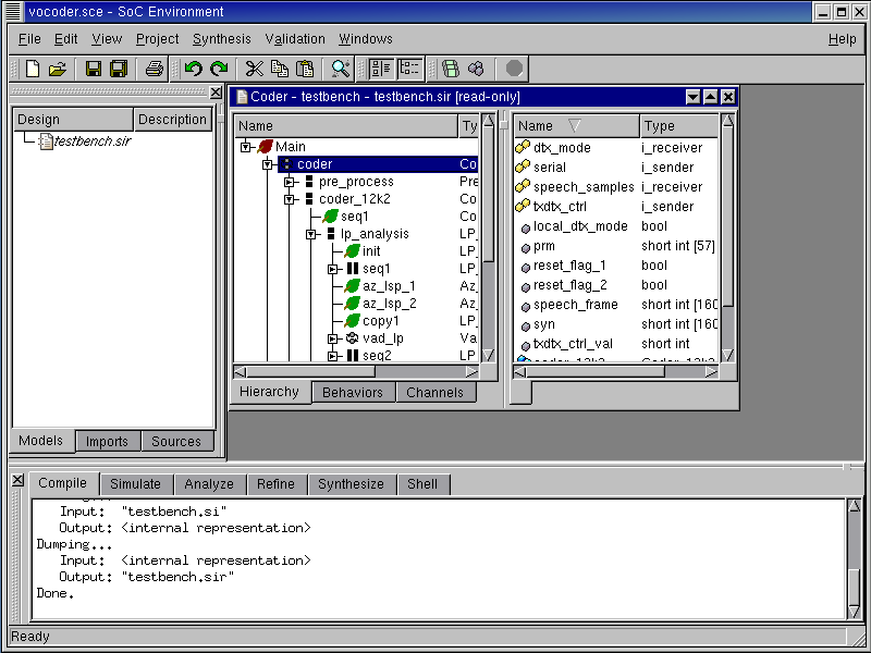
The project is now added as seen in the project management workspace on the left in the GUI.
2.3.1.2. Simulate specification model (cont'd)
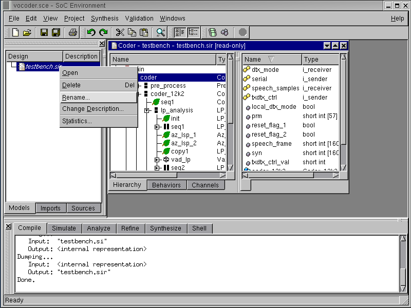
We must now rename the project to have a suitable name. Remember that our methodology involved 4 models at different levels of abstraction. As these new models are produced, we need to keep track of them. Right click on "testbench.sir" and select Rename to rename the design to "VocoderSpec". This indicates that the current model corresponds to the topmost level of abstraction, namely the specification level. Note that the extension ".sir" would be automatically appended. Also note that a model may be made activated, deleted, renamed and and its description modified by right click on its name in the project management window.
2.3.1.3. Simulate specification model (cont'd)
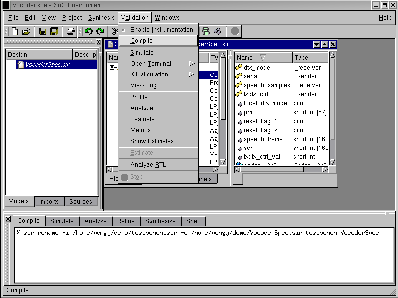
After the project is renamed to "VocoderSpec.sir", we need to compile it to produce an executable. This may be done by selecting Validation->Compile from the menu bar. Note that the validation menu also provides for code instrumentation which is used for profiling. Moreover, we have choices for simulating the model, opening a simulation terminal, killing a running simulation, viewing the log, profiling, analyzing simulation results, model evaluation, displaying metrics and estimates etc. All these features will be used in due course of our system design process.
2.3.1.4. Simulate specification model (cont'd)
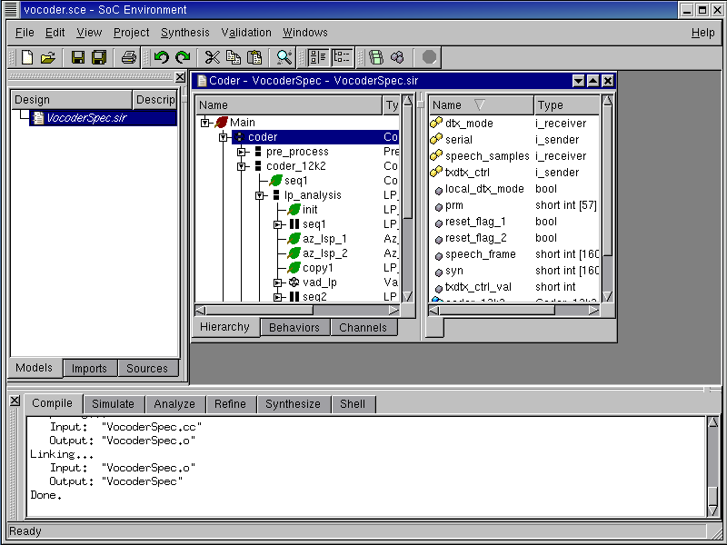
Note that in the logging window we see the compilation messages and an output executable "VocoderSpec" is created.
2.3.1.5. Simulate specification model (cont'd)
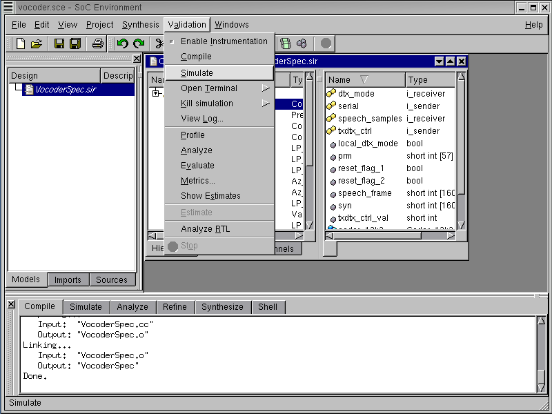
The next step is to simulate the model to verify whether it meets our requirements or not. This may be done by selecting Validation->Simulate from the menu bar.
2.3.1.6. Simulate specification model (cont'd)
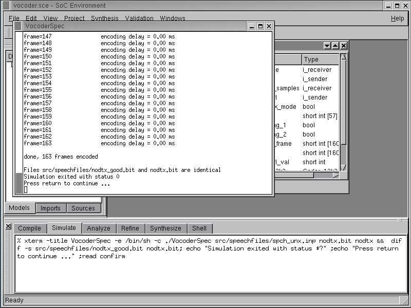
Note that an xterm pops up showing the simulation of the Vocoder specification model on a 163 frame speech sample. The simulation should finish correctly which is indicated by the exit status being '0'. It can be seen that 163 speech frames were correctly simulated and the resulting bit file matches the one given with the vocoder standard. It may be noted that each frame has an encoding delay of 0 ms. This is a because our specification model has no notion of timing. As explained in the methodology, the specification is a purely functional representation of the design and is devoid of timing. For this reason, all behaviors in the model execute in 0 time thereby giving an encoding delay of 0 for each frame. Press RETURN to close this window and proceed to the next step.
2.3.2. Profile specification model
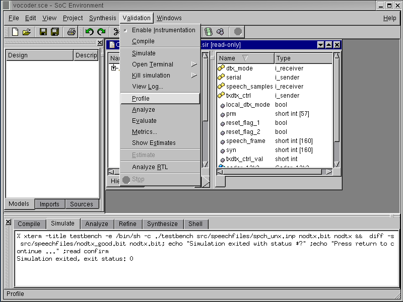
In order to select the right architecture for implementing the model, we must begin by profiling the specification model. Profiling provides us with useful data needed for comparative analysis of various modules in the design. It also counts the various metrics like number of operations, class and type of operation, data exchanged between behaviors etc. These statistics are collected during simulation. Profiling may be done by selecting Validation->Profile from the menu bar.
2.3.2.1. Profile specification model (cont'd)
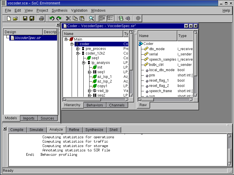
The logging window now shows the results of the profiling command. Note that there is a series of steps for computing statistics for individual metrics like operations, traffic, storage etc. Once these statistics are computed, they are annotated to the model and displayed in the design window.
2.3.2.2. Profile specification model (cont'd)
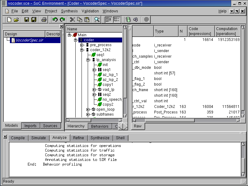
It may also be noted that the design management window now has new column entries that contain the profile data. Maximize this window and scroll to the right to see various metrics for behaviors selected in the design hierarchy. The current screen shot shows Computation, Data, Connections and Traffic for the top level behavior "coder". Computation essentially means the number of operations in each of the behaviors. Data refers to the amount of memory required by the behaviors. Connections indicate the presence of inter-behavior channels or connection through variables. Traffic refers to the actual amount of data exchanged between behaviors. The metrics may also be obtained for other behaviors in the design besides "coder".
2.3.3. Analyze profiling results
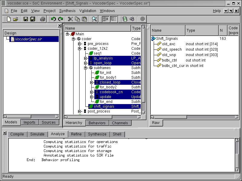
Once we have the profiling results, we need a comparative analysis of the various behaviors to enable suitable partitioning. Here we analyze the six most computationally intensive behaviors namely "lp_analysis", "open_loop", "closed_loop", "codebook_cn", "update" and "shift_signals." They may be multi-selected in the design hierarchy by pressing CNTRL key and left clicking on them. These particular behaviors were selected because these are the major blocks in the behavior "coder_12k2", which in turn is the central block of the entire coder. Thus the selected behaviors show essentially the major part of the activity in the coder. We ignore the pre-processing and the post-processing blocks, because they are of relatively lower importance.
2.3.3.1. Analyze profiling results (cont'd)
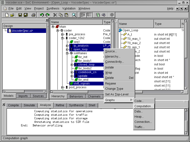
In order to select a suitable architecture for implementing the system, we must perform not only an absolute but also a comparative study of the computation requirements of the selected behaviors. SCE provides for graphical view of profiling statistics which may be used for this purpose. After the multi-selection, we right click and select Graphs->Computation from the menu bar.
2.3.3.2. Analyze profiling results (cont'd)
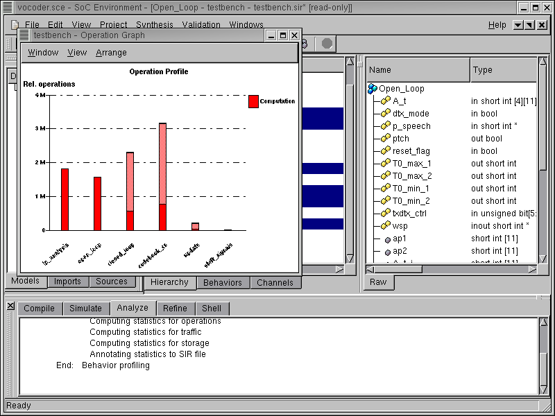
We now see a bar graph showing the relative computational intensity of the various behaviors in the selected behaviors. Essentially, the graph shows the number of operations on the Y-axis for the individual behaviors on the X-axis. Double click on the bar for codebook_cn to view the distribution of its various operations. Note that we select "codebook_cn" because it is the behavior with the most computational complexity.
Note that the bars representing the computation for "codebook_cn" and "closed_loop" have two sections. The lower section is filled with red color and the upper section is partially shaded. Each speech frame consists of four sub-frames and the behaviors "codebook_cn" and "closed_loop" are executed for each subframe in contrast to other behaviors in the graph, which are executed once. Hence the filled section of the bar represents computation for each execution of behavior and the complete bar (including the shaded section) represents computation for the entire frame.
2.3.3.3. Analyze profiling results (cont'd)
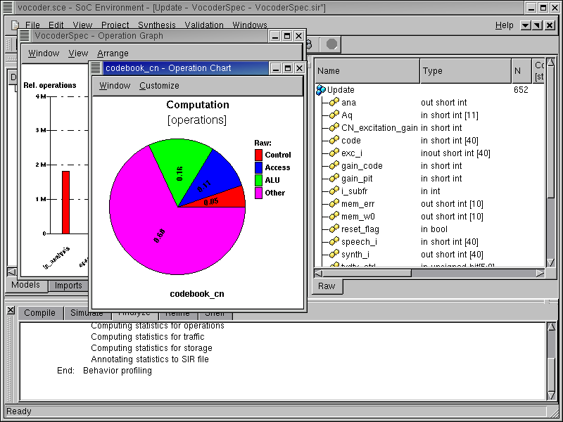
A new window pops up showing a pie chart. This pie chart shows the distribution of various operations like ALU, Control, Memory Access etc. We are interested in seeing the types of ALU operation for this design. To do this double click on the ALU (green) sector of the pie chart.
2.3.3.4. Analyze profiling results (cont'd)
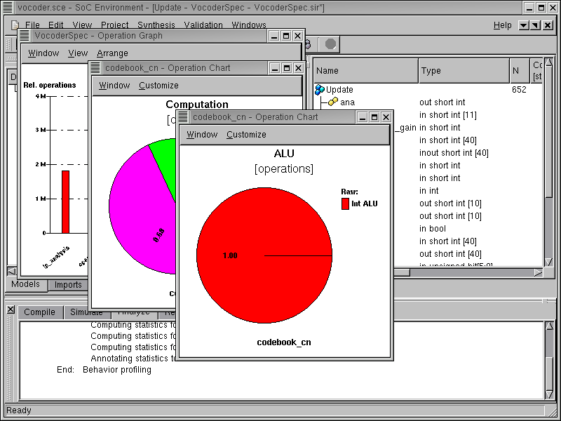
A new window pops up showing another pie chart. This pie chart shows the distribution of ALU operations. It can be seen that all the operations are integer operations, which is typical for signal processing application like the Vocoder. Since all the operations are integral, it does not make sense to have any floating point units in the design. Instead, we need a component with fast integer arithmetic like a DSP. To see the distribution of these integer operations, again double click on the pie chart.
2.3.3.5. Analyze profiling results (cont'd)
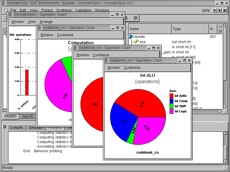
A new window pops up showing another pie chart. This pie chart shows the distribution of the type of integer operations. We can see that the majority of the operations is integer arithmetic. To view the distribution of the arithmetic operation types, again double click on the sector for "Int Arith".
2.3.3.6. Analyze profiling results (cont'd)
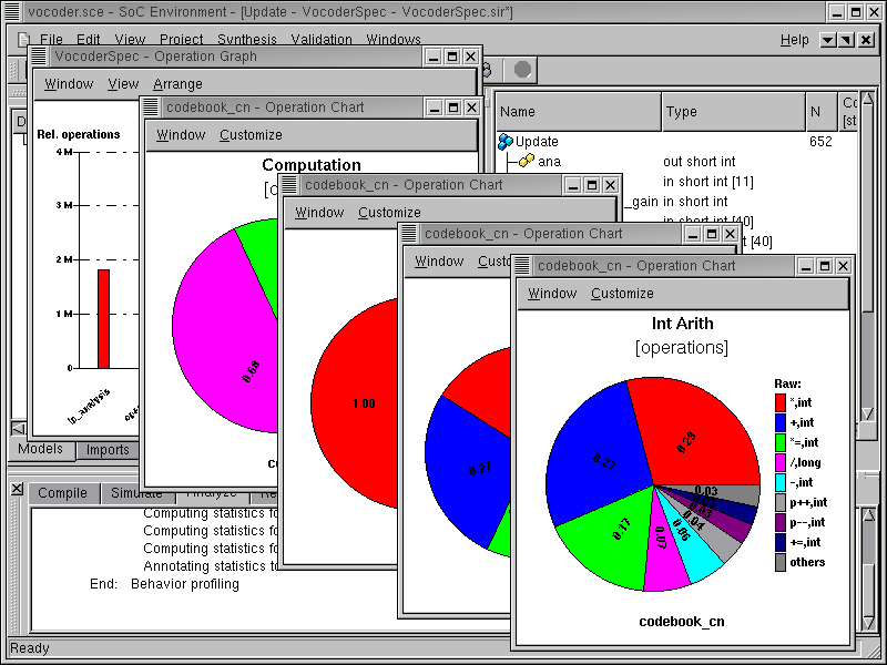
We can now observe the distribution of arithmetic operations like "multiplication", "addition", "increment", "decrement", etc. on a new pie chart. Note that 3 quarters of the operations are additions or multiplications, thus it would be a good idea to have these two operations directly supported by a specific hardware unit.
The combination of visual aids like bar graphs and pie charts gives a good idea of the nature of intended system. Please close all the pop-up windows to conclude the specification analysis phase.